Synopsis

This is a project I did independently to practice my model building skills. This project includes:

• Data exploration and preprocessing using Pandas
• Visualizations using Seaborn and Matplotlib
• String parsing
• Classification Model building using SciKitLearn and XGBoost
• Model tuning using GridSearchCV
• Analysis of model performance using confusing matrix and ROC metrics

The Dataset

The dataset comes from the NASA Open API and NEO Earth Close Approaches. It can be found on Kaggle here: Data. I am using version 2 of this dataset.

This dataset contains information about asteroids orbiting earth. It is important to understand objects close to earth, as they can impact the earth in many ways and distrupt the earths natural phenomena. Information about the size, velocity, distance from earths orbit, and the magnitude of the luminosity of the asteroid can help experts identify whether an asteroid poses a threat or not. This project will analyze information about these asteroids, and attempt to create a model to predict whether or not an asteroid is potentially hazardous.

The attributes of this dataset are:

• id : identifier (the same object can have several rows in the dataset, as it has been observed multiple times)
• name : name given by NASA (including the year the asteroid was discovered)
• est_diameter_min : minimum estimated diameter in kilometers
• est_diameter_max : maximum estimated diameter in kilometers
• relative_velocity : velocity relative to earth
• miss_distance : distance in kilometers it misses Earth
• orbiting_body : planet that the asteroid orbits
• sentry_object : whether it is included in sentry - an automated collision monitoring system
• absolute_magnitude : intrinsic luminosity
• hazardous : whether the asteriod is potentially harmful or not

Exploratory Data Analysis and Pre-processing

This dataset has 10 columns and 90,836 rows. It has no missing values. Peeking at the first 10 rows of data reveals what the data looks like:

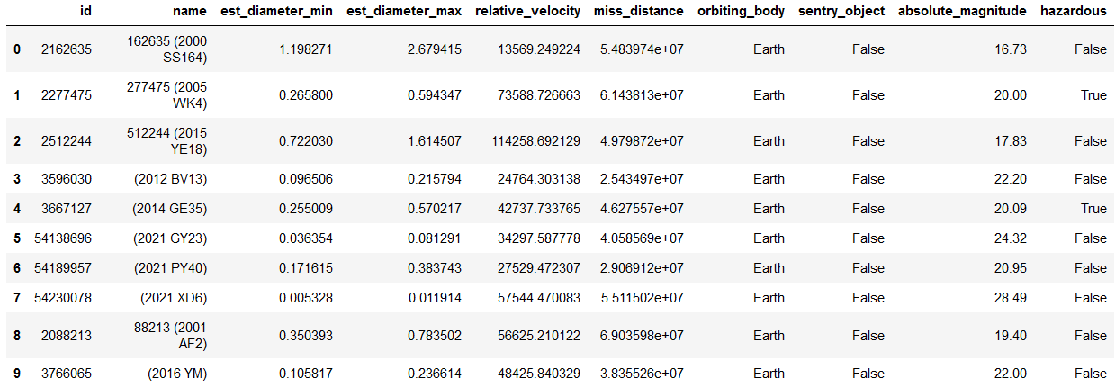
Table 1

A cursory examination of the dataset shows that orbiting_body and sentry_object each only have 1 unique value, so they are dropped from the table.

We also see that id and name each only have 27,423 unique values. This means that the same asteroid is measured multiple times. Let’s take a look at one of these asteroids to see what changes with each record:

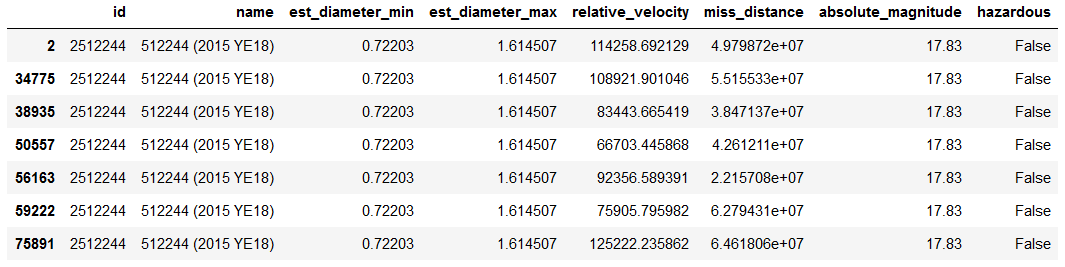
Table 2

Looking at Table 2, it appears that relative_velocity and miss_distance change with each observation of the same asteroid. A large majority of the time, the classification of hazardous does not change with each observation.

We would assume intuitively that most of these asteroids are not hazardous, because if most asteroids were hazardous we would probably have a lot more collisions with them! The imbalance is not too extreme though- about 9.7% of objects are classified as hazardous. This can be handled with a stratified train-test split later on.

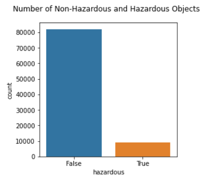
Figure 1

Next, a correlation heatmap in Figure 2 shows that est_diameter_min and est_diameter_max are perfectly correlated. This means we only need to keep one of these variables, so we will drop est_diameter_min.

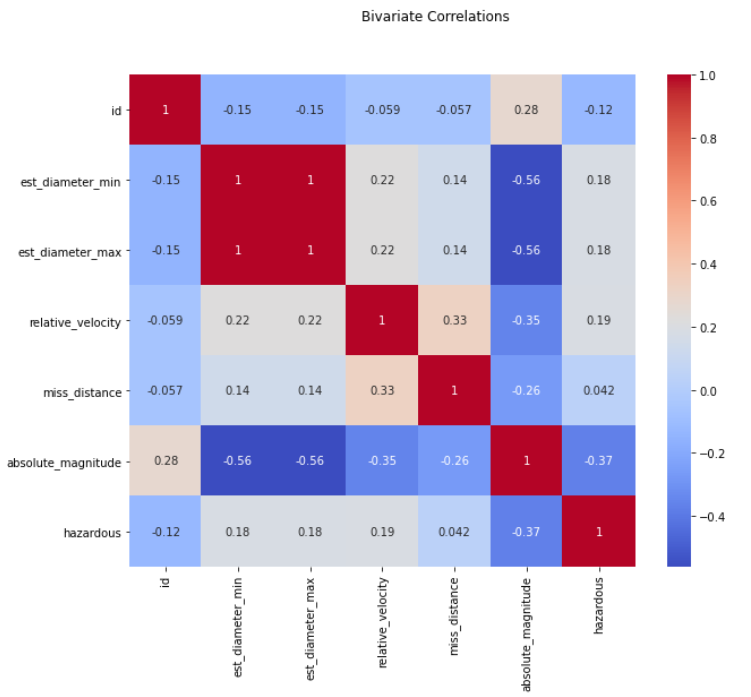
Figure 2

Next, I was curious about the year that is included in the names of each asteroid. I decided to extract the year from the name variable to see if there is any pattern with the year the asteroid was discovered.

df[['drop','temp']]=df.name.str.split('(',expand=True)
df.drop(columns='drop',inplace=True)

def get_year(x):
    return x.strip()[0:x.strip().index(' ')]
df['year']=df['temp'].apply(get_year)

df.drop(columns='temp', inplace=True)

df.loc[df.year=='A911','year']='1911' 
df.loc[df.year=='6743','year']='1960'
df.loc[df.year=='A898','year']='1898'
df.loc[df.year=='6344','year']='1960'
df.loc[df.year=='A924','year']='1924'
df.loc[df.year=='A/2019','year']='2019'
df.loc[df.year=='4788','year']='1960'
  
df.year=df.year.astype(int)

To see if there is any pattern, I created boxplots for hazardous and non-hazardous asteroids based on the year. Based on the boxplots in figure 3, hazardous objects were mostly discovered between around 2002 to before 2020. There were many non-hazardous objects discovered pre-1980s.

Possible reasons why hazardous objects were not discovered until more recently could be that hazardous asteroids tend to be farther away (as we will discover from figure 5), and it is possible that older equipment could not detect asteroids that are further away from earth as well. Another possible reason is that hazardous objects tend to have a lower absolute magnitude (also infered from figure 5), or luminosity, making them even harder to detect with older equipment.

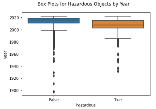
Figure 3

Univariate and Bivariate Analysis

To perform univariate and bivariate analysis, I began by extracting the numerical columns, not including id.

First I checked the distribution of the variables, shown in figure 4. First, notice that the distribution for estimated maximum diameter is highly positively skewed with sharp spike on the left, indicating the presence of outliers. Relative velocity has a positive skew, so most asteroids are moving more slowly. The distance from earth, miss_distance, seems to be relatively uniform throughout the data, with a bit of a spike at 0. Finally, we see that most observations of asteroids were recorded after 1990, so data from before 1990 might not be as useful.

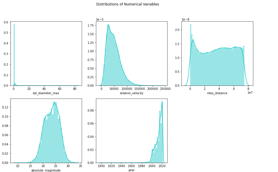
Figure 4

For bivariate analysis, I started with a pairs plot that is colored by hazardous classification (figure 5). There are a lot of interesting patterns revealed by these plots.

First, the distributions along the diagonal are interesting because they add more information to our univariate analysis concerning the classification of asteroids as hazardous. From the relative velocity distribution, it seems that hazardous asteroids move slightly faster than non-hazardous ones. From the distributions of miss_distance and absolute_magnitude, we see that hazardous asteroids actually tend to be further away from earth, which is counter-intuitive. There is also a very clear correlation between est_diameter_max and absolute_magnitude, so it may be beneficial to only include one of these variables for certain models.

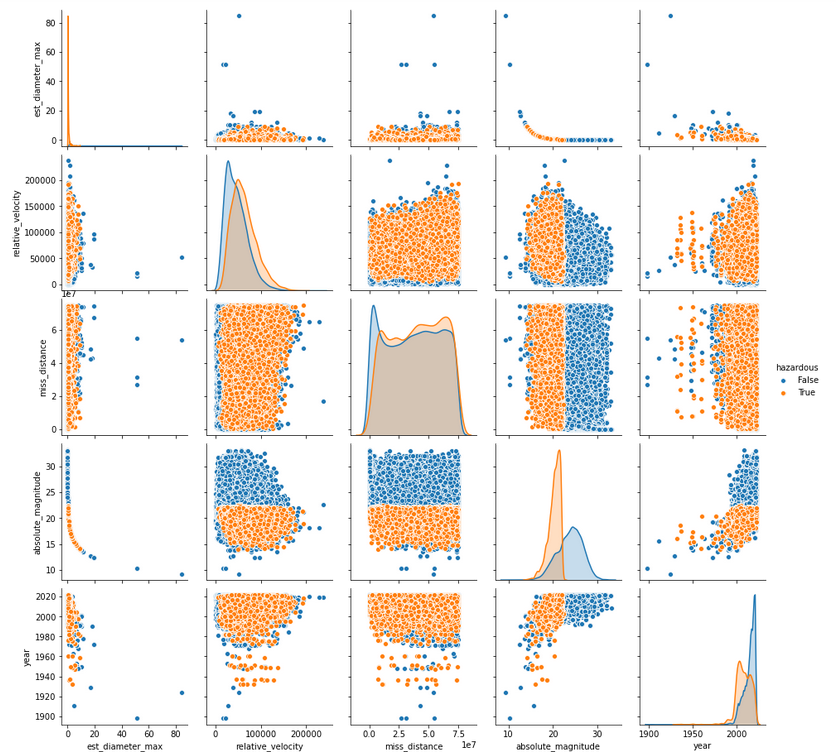
Figure 5

num_cols = ["est_diameter_max", "relative_velocity", "miss_distance", "absolute_magnitude","year"]

rows=2
cols=3
count=1
plt.rcParams['figure.figsize']=[15,9]
for i in num_cols:
    plt.subplot(rows,cols,count)
    sns.distplot(df[i], color='c')
    count+=1
plt.suptitle('Distributions of Numerical Variables')
plt.show()

sns.pairplot(df[num_cols+['hazardous']],hue = 'hazardous')

Model Building

I chose to create classification models to predict whether or not an asteroid is considered hazardous. To compare models, I included accuracy, precision, recall, f1, and AUC scores. I chose to include all of these metrics because certain models performed better for some of these metrics and worse for others. In this case, recall is going to be more important than precision (or even accuracy, to a degree) because mis-classifying a dangerous asteroid as non-hazardous is a much more costly mistake that mis-classifying a non-hazardous asteroid. So, if a model performs better in recall and worse for other metrics, it may be something to take into account.

More Pre-Processing

Before building any models, I performed a test/train split, with 80% of the data going to the test set. I stratified y (the hazardous variable) to account for the class imbalance. I did not include name or id in the X values because they were not useful. I decided to keep both estimated_diameter_max and absolute_magnitude, because most of the metrics were improved by including both variables. However, if we were trying to optimize recall only, it would help with certain models to only use one of these variables.

Next, I transformed my X variables using StandardScaler from the SKLearn library. This was necessary mostly for k-nearest neighbors classification, as it uses euclidian distance and the magnitudes of the X variables were all very different.

Finally, I created a function for plotting a ROC curve for each of the classification models. This helped to reduce redundant code.

X = df.drop(["id","name","hazardous"], axis=1)
y = df.hazardous.astype(int)
    
X_train, X_test, y_train, y_test = train_test_split(X,y, test_size = 0.2, random_state = 0, stratify=y)
    
sc=StandardScaler()
X_train_scaled=pd.DataFrame(sc.fit_transform(X_train))
X_test_scaled=pd.DataFrame(sc.transform(X_test))
    
def roc_curve_plot(y_test, y_scores, method):
    fpr, tpr, threshold = roc_curve(y_test, y_scores[:, 1])
    roc_auc = auc(fpr, tpr)
    plt.plot(fpr, tpr, 'b', label = 'AUC = %0.2f' % roc_auc)
    plt.legend()
    plt.plot([0, 1], [0, 1],'r--')
    plt.ylabel('True Positive Rate')
    plt.xlabel('False Positive Rate')
    plt.title('ROC Curve of ' + method)
    plt.rcParams['figure.figsize']=[6,5]
    plt.show()
    return roc_auc

Basic Decision Tree Classification

I knew the basic decision tree classifier would not be the most accurate, however I thought it would be a good starting point to compare our other models against. It is also a good way to get a basic idea of how important each variable is to the decision tree, and to compare an importance plot to our other tree methods.

The decision tree ended up being too large to be especially helpful. The models scores are shown in table 3 below. I also plotted the ROC curve for the model, which shows that it is a decent model compared to a random model, but certainly not good enough for predicting hazardous asteroids.

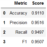
Table 3

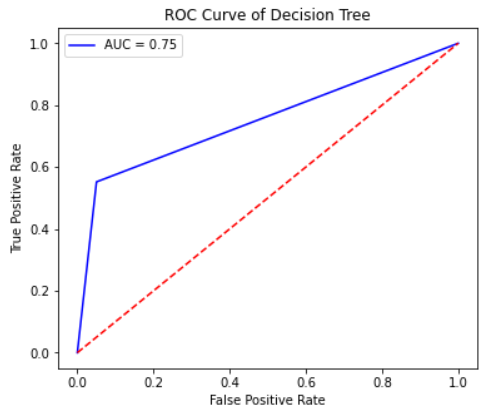
Figure 6

I plotted the variable importance for all of the tree-based models. The importance for each variable is shown in figure 7. This decision tree model mainly uses the diameter to classify the objects, which is interesting because the diameter does not vary much between asteroids. The variables miss_distance and relative_velocity are also important variables in this tree, which makes sense with the correlations we saw in figure 5 between those two variables and the hazardous classification.

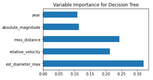
Figure 7

DT = DecisionTreeClassifier()
tree = DT.fit(X_train_scaled, y_train)
DT_pred = DT.predict(X_test_scaled)
Acc_DT = round(accuracy_score(DT_pred, y_test), 4)
xgprec_DT, xgrec_DT, xgf_DT, support_DT = score(y_test, DT_pred)
precision_DT, recall_DT, f1_DT = round(xgprec_DT[0], 4), round(xgrec_DT[0],4), round(xgf_DT[0],4)
scores_DT = pd.DataFrame({
    'Metric': ['Accuracy', 'Precision', 'Recall', 'F1'],
    'Score': [Acc_DT, precision_DT, recall_DT, f1_DT]})
scores_DT
    
y_scores_DT = DT.predict_proba(X_test_scaled)
auc_DT = roc_curve_plot(y_test, y_scores_DT, 'Decision Tree')
    
feat_importances = pd.Series(DT.feature_importances_, index=X.columns)
feat_importances.plot(kind='barh', title='Variable Importance for Decision Tree',figsize=[5,3])

K Nearest Neighbors Classification

Next I wanted to try K Nearest Neighbors because I wanted a model that was not tree-based, and I figured clustering makes sense because intuitively, you would expect asteroids that are similar to have the same classification. I was surprised by how well it performed. I used the elbow method to choose k, and based on figure 8 I chose k=15.

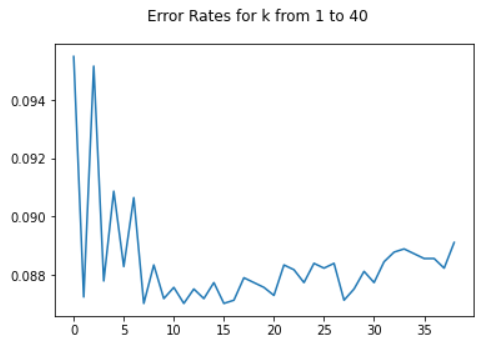
Figure 8

K Nearest Neighbors performed much better than the decision tree, but an accuracy of 91% still is not quite as high as we would like, considering the importance of classifying asteroids correctly. The recall is fairly high which is especially important. Overall, this model is good, but not up to NASA standards.

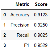
Table 4

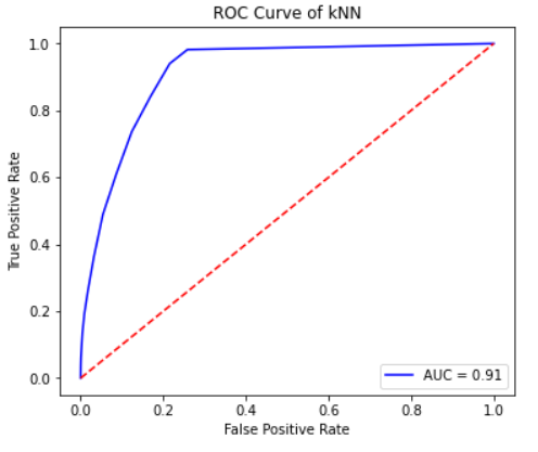
Figure 9

error_rates = []
for i in np.arange(1, 40):
    model = KNeighborsClassifier(n_neighbors = i)
    model.fit(X_train_scaled, y_train)
    predictions = model.predict(X_test_scaled)
    error_rates.append(np.mean(predictions != y_test))

plt.rcParams['figure.figsize']=[6,4]
plt.suptitle('Error Rates for k from 1 to 40')
plt.plot(error_rates)
    
KNN = KNeighborsClassifier(n_neighbors = 15)
KNN.fit(X_train_scaled, y_train)
KNN_pred = KNN.predict(X_test_scaled)
Acc_KNN = round(accuracy_score(KNN_pred, y_test), 4)
xgprec_KNN, xgrec_KNN, xgf_KNN, support_KNN = score(y_test, KNN_pred)
precision_KNN, recall_KNN, f1_KNN = round(xgprec_KNN[0], 4), round(xgrec_KNN[0],4), round(xgf_KNN[0],4)
scores_KNN = pd.DataFrame({
    'Metric': ['Accuracy', 'Precision', 'Recall', 'F1'],
    'Score': [Acc_KNN, precision_KNN, recall_KNN, f1_KNN]})
scores_KNN
    
y_scores_KNN = KNN.predict_proba(X_test_scaled)
auc_KNN = roc_curve_plot(y_test, y_scores_KNN, 'kNN')

Random Forest Classification

For the next model, I decided to try Random Forest to improve on the decision tree model. I knew this would perform better than the basic decision tree. Random Forest ended up having the best AUC, Accuracy, and F1 scores out of all the models I created.

Hyperparameter tuning using GridSearch showed that the default settings were sufficient, although recall can be improved slightly by using max_depth=16 and n_estimators= 256 for the models parameters. I decided to keep the default parameters to improve all other metrics. The accuracy for this model, shown in table 5, is close to 93%. This is the best accuracy I was able to get from any of the models. The AUC is also very high for this model, as shown in figure 10.

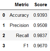
Table 5

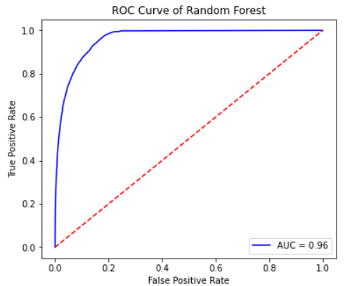
Figure 10

Finally, I wanted to see the variable importance plot for random forest, shown in figure 11. I found it very interesting that all the variables are very close to each other in importance. The diameter and miss distance variables are still both the most important, but relative velocity and absolute magnitude are still very important compared to the basic decision tree.

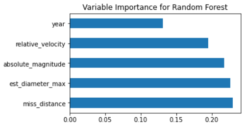
Figure 11

max_depth=[2, 8, 16]
n_estimators = [64, 128, 256]
param_grid = dict(max_depth=max_depth, n_estimators=n_estimators)
dfrst = RandomForestClassifier(n_estimators=n_estimators, max_depth=max_depth)
grid = GridSearchCV(estimator=dfrst, param_grid=param_grid, cv = 5)
grid_results = grid.fit(X_train_scaled, y_train)

print("Best: {0}, using {1}".format(grid_results.cv_results_['mean_test_score'], grid_results.best_params_))
    
RF = RandomForestClassifier()
RF.fit(X_train_scaled, y_train)
RF_pred = RF.predict(X_test_scaled)
Acc_RF = round(accuracy_score(RF_pred, y_test), 4)
xgprec_RF, xgrec_RF, xgf_RF, support_RF = score(y_test, RF_pred)
precision_RF, recall_RF, f1_RF = round(xgprec_RF[0], 4), round(xgrec_RF[0],4), round(xgf_RF[0],4)
scores_RF = pd.DataFrame({
    'Metric': ['Accuracy', 'Precision', 'Recall', 'F1'],
    'Score': [Acc_RF, precision_RF, recall_RF, f1_RF]})
scores_RF
    
y_scores_RF = RF.predict_proba(X_test_scaled)
auc_RF = roc_curve_plot(y_test, y_scores_RF, 'Random Forest')
    
feat_importances_RF = pd.Series(RF.feature_importances_, index=X.columns)
feat_importances_RF.nlargest(8).plot(kind='barh', title = 'Variable Importance for Random Forest', figsize=[5,3])

Gradient Boosted Decision Tree Classification

The last model I chose to create is a gradient boosted decision tree from the Extreme Gradient Boosted Classifier model from the XGBoost library. This method has gained a lot of popularity through its performance in Kaggle competitions, so I wanted to see how it would perform on this dataset. The gradient boosted machine did not need hyperparameter tuning in this case.

Overall, the gradient boosted decision tree performed nearly as well as the random forest. All of the metrics from table 6 are just slightly less than those for the random forest model, with the exception of recall. The gradient boosted classifier outperformed the random forest model in recall by a little bit. However, because we know recall is an important metric in this specific case due to the consequences of a false negative, the decision maker may prefer to sacrifice accuracy and precision a little bit to improve recall.

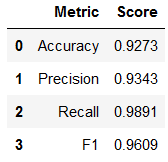
Table 6

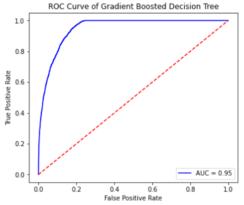
Figure 12

The variable importance plot for the gradient boosted machine is very interesting. It is almost opposite of the variable importance plot for random forest. It values the diameter variable the most, just like in the other plots, but all other variables are much less important. It does not even appear to use the absolute magnitude at all. It is interesting how different this variable importance plot is compared to random forest, considering how similarly the two models performed.

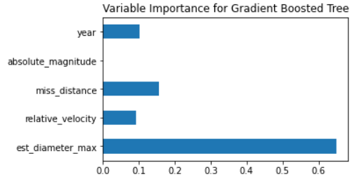
Figure 13

XGB = XGBClassifier()
XGB.fit(X_train_scaled, y_train)
XGB_pred = XGB.predict(X_test_scaled)
Acc_XGB = round(accuracy_score(XGB_pred, y_test),4)
xgprec_XGB, xgrec_XGB, xgf_XGB, support_XGB = score(y_test, XGB_pred)
precision_XGB, recall_XGB, f1_XGB = round(xgprec_XGB[0], 4), round(xgrec_XGB[0],4), round(xgf_XGB[0],4)
scores_XGB = pd.DataFrame({
    'Metric': ['Accuracy', 'Precision', 'Recall', 'F1'],
    'Score': [Acc_XGB, precision_XGB, recall_XGB, f1_XGB]})
scores_XGB
    
y_scores_XGB = XGB.predict_proba(X_test_scaled)
auc_XGB = roc_curve_plot(y_test, y_scores_XGB, 'Gradient Boosted Decision Tree')
    
feat_importances_XGB = pd.Series(XGB.feature_importances_, index=X.columns)
feat_importances_XGB.plot(kind='barh', title = 'Variable Importance for Gradient Boosted Tree', figsize=[5,3])

Final Results and Remarks

Overall, it is clear that both Random Forest classification and Gradient Boosted classification outperformed the Decision Tree and K Nearest Neighbors. I was very impressed with how accurate both the Random Forest and Gradient Boosted models were. They both had very high AUC, accuracy, and recall scores. As I’ve mentioned, recall is especially important in this case. Decision makers using these models would need to decide if the slight increase in recall for the Gradient Boosted model over the Random Forest model is worth sacrificing a little bit of accuracy and AUC. However, I believe either model would be a good choice.

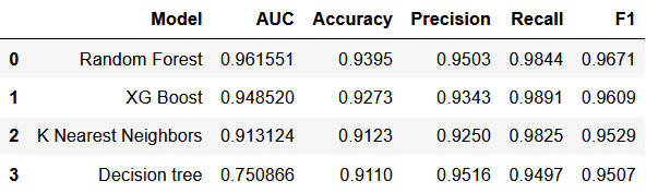
Table 7

The variable importance plots revealed that the diameter of an asteroid is the main predictor of its danger. This is inutitive, but it is not obvious from the univariate and bivariate analyses. The importance plots also show that the distance from the earth (miss_distance) is also very important, although we learned from the bivariate analysis that the asteroids that are further away are actually more dangerous than the ones closer to earth. We also see from the variable importance plots that the year the asteroid was discovered does impact its hazard classification, possibly due to changing technology at NASA.

I do feel this project was successful in creating fairly accurate and useful models to predict the danger an asteroid near earth poses. It revealed a lot of interesting facts about asteroids, and I would be interested in continuing to improve these models over time.

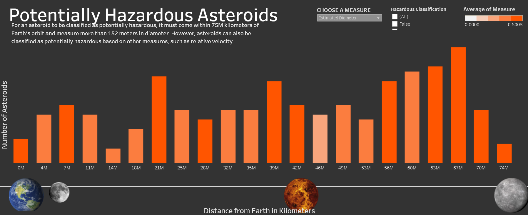
Tableau Dashboard

Click here to see the interactive dashboard

I created an interactive visualization using Tableau for this dataset. The visualization is a bar graph showing how many asteroids are certain distances from Earth. The colors of the bars are associated with realtive velocity or estimated diameter, selected by the user. The user can also choose to include only hazardous asteroids, only non-hazardous asteroids, or all asteroids. The bottom of the visualization shows references for the distance of other planets from Earth.

This visualization reveals some rather interesting patterns. One thing we see is that most of the near-earth asteroids are located within 20 million kilometers of Earth. However, most of the hazardous near-earth asteroids are between 55-70 million kilometers away. When looking at relative velocity, we can see that for all near-earth asteroids, the ones further away from Earth tend to have a slightly higher velocity. Diameter seems to be highly correlated with distance from Earth, there is a very clear pattern that larger asteroids tend to be further from Earth.

Thank you so much for reading my project. I appreciate your time. If you have any advice for improving this project, I would love to hear it! Please email me at ahowe615@gmail.com with any comments.