This is my final project for Stats 515 at George Mason University. This project was done entirely in R.
Wine is a complex product with many facets that contribute to taste and quality. Understanding the major factors that attribute most to the quality of a wine is an important business analysis issue. My project attempts to understand what attributes impact the quality of a wine and how one can predict a wine’s quality by performing exploratory data analysis, variable subset selection, and creating multiple classification models.
The Dataset
The dataset comes from the UCI Machine Learning Repository (Data).
This dataset, from the University of California, Irvine machine learning repository, was collected between 2004-2007. It focuses specifically on the vinho verde red wine from Portugal. Each wine was assessed in a laboratory for 11 different physicochemical features. Then, a quality score from 1 to 10 was derived by measuring the median of a minimum of three blind sensory tests conducted by wine experts.
The attributes of this dataset are:
- Alcohol percentage
- Volatile acidity
- Citric acid
- Fixed acidity
- Residual sugar
- Density
- pH
- Free sulfur dioxide
- Total sulfur dioxide
- Chlorides
- Sulphates
- Quality
Exploratory Data Analysis
Table 1 shows a summary of all the variables. There are no quality scores below 3 or above 8, so there’s no really high or low quality wines. This may skew results because there’s no data on the makeup of a “perfect” wine.
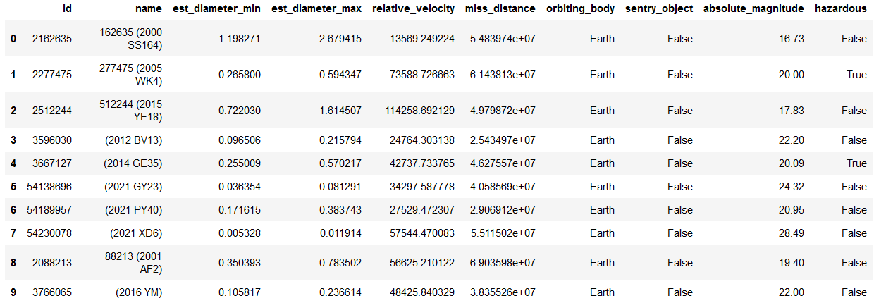
Table 1
A histogram of the quality scores shows the distribution of the dependent variable in Figure 1. This shows that a large majority of the scores lie between 4 and 6, so most of the wines included in the dataset are of average quality. The lack of data for very low and very high-quality wines may mean the models created from this dataset are less robust to added instances.
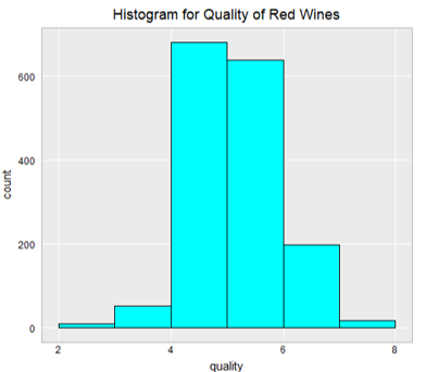
Figure 1
The scatterplot matrix in Figure 2 shows the distributions of all variables along the diagonal and a scatterplot for each pair of variables with a smooth showing the correlation between the pairs. A few variables have very skewed distributions, including residual sugar, chlorides, free sulfur dioxide, total sulfur dioxide, and sulphates. These variables will benefit from a log transformation to fix the skew later.
Other important aspects of Figure 2 are the pairs of variables with strong correlations. Variables that are correlated with each other include all of the acid variables, fixed acidity and density, fixed acidity and pH, and chlorides and sulphates.
Variables that are strongly correlated with quality based on the scatterplot matrix are volatile acidity (which makes the wine taste like vinegar when high), sulphates, and alcohol percentage. This is the first indication that these variables may be strong predictors of quality.
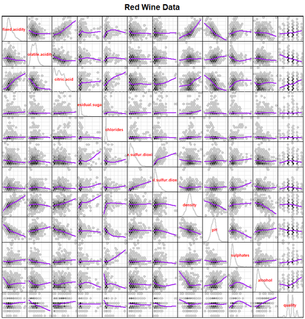
Figure 2
For the final aspect of the exploratory data analysis, I created a 3D interactive scatterplot using the plotly library in Figure 3. The axes are the three variables showing a strong correlation with quality: alcohol percentage, volatile acidity, and sulphates. The colors are based on the quality score.
Most of the higher-quality wines are grouped together on the left side of the plot, with higher alcohol levels, lower volatile acidity, and moderate to high sulphate levels. This graphic also shows that outliers tend to have lower quality scores. Very high or low values for any one of the variables make the wine less desirable.
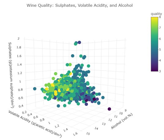
Figure 3
Variable Selection
In the scatterplot matrix in Figure 2, the bottom row of scatterplots shows the correlations of each variable with quality score. Not all the independent variables are correlated with quality, so not all of them will be useful in classifying the wines. I tried several methods to find the best subset of variables to classify and predict quality score.
I began by running best subset selection with a maximum of 10 variables included using the leaps package. To choose an appropriate number of variables to include in the subset, I plotted the residual sum of squares and adjusted R2 versus the number of variables (Figure 4). The plots show that both RSS and R2 start to level off at about six variables, so that is a reasonable choice for the number of variables to include in the subset.
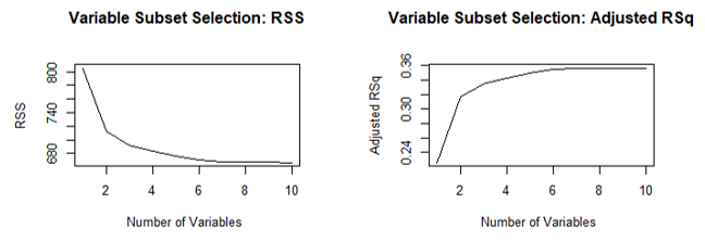
Figure 4
The best subset selection method, forward, and backward stepwise selection all produced the same results. As shown in Figure 5, the six variables that should be included are volatile acidity, chlorides, total sulfur dioxide, pH, sulphates, and alcohol percentage.
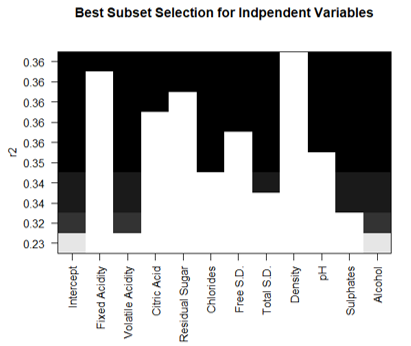
Figure 5
Tree Based Models
The first set of classification models I created are two different tree-based models: the basic classification tree and random forest regression. I created a new binary variable which indicates whether a wine is good quality or not. A wine is good quality if it has a quality score of 6 or higher. Both models were created using a training set and validated using a test set, with a 75-25 split. The goal of the models is to classify a wine based on its physiochemical features.
Basic Classification Tree
Starting with the basic classification tree using the six-variable subset identified in the previous section, I created the tree using the rpart package.
Results
A graph of the basic classification tree is shown in Figure 6. Running the decision tree on the test set resulted in a p-value of 3.973e-16 for the model, which shows statistical significance. The accuracy based on the confusion matrix is 73%.
The variable importance output showed that alcohol percentage was the most important variable, and chlorides and pH level were the least important variables. The classification tree is a valid one, even though it could be more accurate.
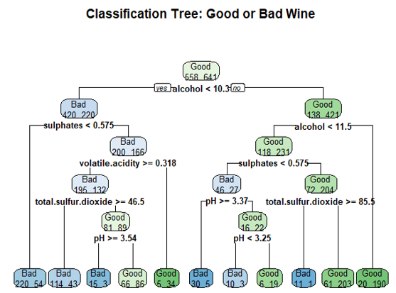
Figure 6
Random Forest Regression Model
The other tree-based model is a random forest regression model using the randomForest package. In this one, all 11 independent variables are included to provide a more accurate variable importance plot. I used the default of 500 trees and 3 variables at each split.
Results
The out-of-bag error estimate from the training set model is 20%, and the accuracy for the test model is 85%, which is a significant improvement over the basic classification tree. The model’s p-value is less than 2e-16 which shows statistical significance.
The variable importance plot in Figure 7 indicates that the six most important variables according to the random forest model are nearly the same as the six variables chosen in the best subset selection methods, with density replacing pH in the top six. This indicates that pH is one of the weaker predictors of quality as compared to alcohol, sulfates, and volatile acidity.
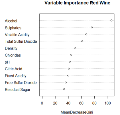
Figure 7
Logistic Regression Model
Because the predictor variable is binary, I tried logistic regression to see if it would perform better than the random forest regression model.
Before performing logistic regression, I log-transformed several of the skewed variables, including residual sugar, chlorides, free sulfur dioxide, total sulfur dioxide, and sulphates. Then I created a logistic regression model using the six variables identified in the best subset selection.
Results
From the p-values for the independent variables shown in the output, pH is not identified as significant with a p-value of about 0.89. This makes sense as pH was also not included in the six most important variables for random forest regression. The p-value for the model based on the test set is less than 2e-16, which shows statistical significance. The accuracy is 75%, which is better than the basic classification tree but not as accurate as the random forest regression.
I created an effects graph from the effects package to show how each variable affected the logistic regression model. The plot for pH is on the bottom left of the graphic. From this effects graph, it appears that the quality correlation is weak. The blue shading indicates that for low and high pH values, there are large confidence intervals. This most likely is due to the fact that most wines have a pH value near 3.4; the further away from 3.4 the pH value is, the less confident the model is in its prediction. There may be an advantage to leaving out pH.
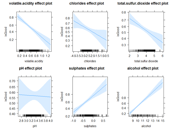
Figure 8
Clustering Model
The last classification model is a cluster analysis using k-means clustering. I expected that performing k-means clustering with two clusters would result in one cluster of bad wines and one of good wines.
Results
Running k-means classification from the cluster package didn’t have a great degree of accuracy. The first cluster, which is highlighted in red in Figure 8, was 64% bad wines, and the second cluster, highlighted in blue, is 59% good wines. Most outliers are included in the first cluster. From the exploratory data analysis, we know that outliers tend to be bad wines, which is possibly why cluster 1 contains a majority of bad wines. This was not an efficient model for this dataset.
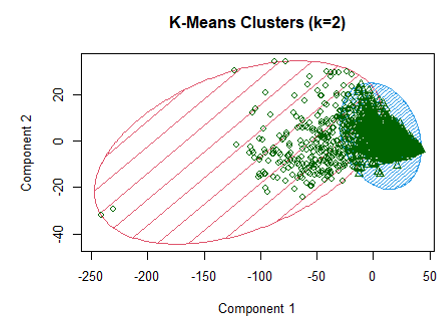
Figure 9
Final Remarks
- The most important factors contributing to quality for red wine are alcohol percentage, volatile acidity, sulphates, chlorides, and total sulfur dioxide. These are consistently the strongest predictors for each type of model. Density and pH are weaker predictors, as each were identified as important for some models and not others.
- Of all the models, random forest regression was the most accurate and statistically significant. Logistic regression performed slightly better than the basic decision tree but was more statistically significant. Cluster analysis was not very successful at clustering good and bad wines together and may have been skewed by outliers.
Overall, based on the strongest predictors and their correlation with quality score, it seems that more alcoholic, less sweet, and lower acidity wines are more favored in quality testing.